2.9. Numerical Stability

Here we will consider the potential accuracy of solutions to systems of equations of the form \(\mathbf{A}\,\bm{x} = \bm{b}\). In idealistic mathematical notation, we write the solution to a square matrix system of equations as \(\bm{x} = \mathbf{A}^{-1}\bm{b}\). However, the path toward finding the true \(\bm{x}\) is fraught with potential problems.

Sometimes it may be difficult to find an accurate solution. It might be that the values in \(\bm{b}\) and \(\bf{A}\) are not accurate because they came from an experiment where noise in the data is unavoidable. It might be that the rows of \(\bf{A}\) are close to parallel, meaning that \(\bf{A}\) is nearly singular—also called poorly conditioned. It might also be that the absolution values of the numbers in \(\bm{b}\) and \(\bf{A}\) are likely to incur round-off errors because they contain a mixture of very large numbers, very small numbers, and even some irrational numbers and numbers that, in binary, contain unresolved repeating patterns of 1’s and 0’s.

Using an algorithm that is not numerically stable leads to inaccurate solution estimates. Numerical stability is a property of the algorithm rather than the problem being solved. The best algorithms might not always find accurate results in the worst conditions. However, numerically stable algorithms find accurate results for most problems. Numerically stable algorithms order the operations on numbers to minimize round-off errors. They also avoid computations that will tend to degrade the condition of matrices. For example, our idealistic mathematical solution to an over-determined system of equations calls for three matrix multiplications, a matrix inverse, and a matrix–vector multiplication. We will see in this section that such a sequence of operations is not advisable. We already know that the matrix inverse is slow. The matrix multiplications can also introduce round-off errors.

After reviewing the source of round-off errors and the condition number of matrices, we will look at three case studies where modified algorithms led to improved numerical stability. Then, in the next section, we will see how orthogonal matrix factoring provides the tools needed for numerically stable solutions to rectangular systems of equations.

2.9.1. Round-off Errors

Round-off errors usually occur when adding or subtracting a small number from a large number. The source of the degraded precision is the finite number of binary bits used to hold the digits of floating-point numbers. Addition or subtraction can cause the less significant binary digits of small numbers to be removed. When the precision of a number is reduced, a round-off error is introduced into the calculations.

The IEEE Standard for Binary Floating-Point Arithmetic [IEEE85] specifies the format of 32-bit single precision and 64-bit double precision floating point numbers. We will focus on the double precision format because most scientific numeric calculations use double data type variables that correspond to the double precision standard. Floating point numbers are stored in a format similar to scientific notation, except that the binary number system (base 2) is used instead of decimal. As shown in equation (2.19), the binary numbers are normalized with adjustments to the exponent so that there is a single 1 to the left of the binary point. The binary digits of the number are called the mantissa. Since the digit to the left of the binary point is always 1, it is not necessary to store that 1. The digits to the right of the binary point are called the significand. As shown in figure Fig. 2.20, double precision numbers store 52 binary digits of the significand. In equation (2.19), the significand is the binary digits \(b_{51}b_{50}\ldots b_0\). Including the 1 to the left of the binary point, the level of available precision in double data type variables is \(u = 2^{-53} \approx 1.11 \times 10^{-16}\) [IEEE85].

(2.19)\[\begin{split}\begin{array}{l} (-1)^{sign} \times (1.b_{51}b_{50}\ldots b_0)_2 \times 2^{exp - 1023}\\ \text{or} \\ mantissa \times 2^{exponent} \end{array}\end{split}\]

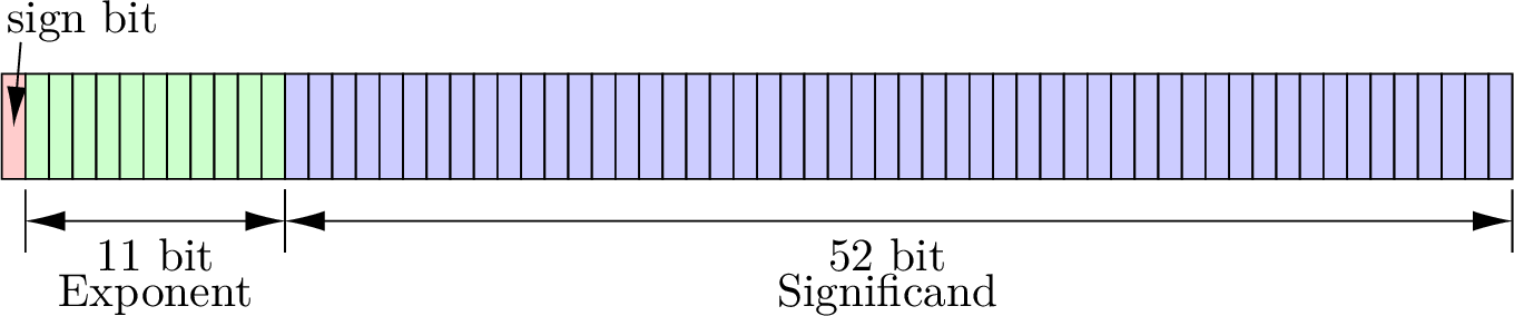
Fig. 2.20 The format of 64-bit double precision floating point numbers.

Let \(x_1 = mantissa_1 \times 2^{exponent_1}\) and let \(x_2 = mantissa_2 \times 2^{exponent_2}\). Further, let \(x_1\) be much greater than \(x_2\), (\(x_1 \gg x_2\)). The exponents are added in multiplication,

\[x_1 \times x_2 = mantissa_1 \times mantissa_2 \times 2^{(exponent_1 + exponent_2)}.\]

Division is a similar process, except the exponents are subtracted. Multiplication and division are immune to numerical problems except in the rare event of overflow or underflow.

Addition and subtraction require that the exponents match.

\[\begin{split}\begin{split} x_1 \,\pm\, x_2 &= mantissa_1 \times 2^{exponent_1} \pm \\ & \quad \left(mantissa_2 \times 2^{(exponent_2 - exponent_1)}\right) \times 2^{exponent_1}. \end{split}\end{split}\]

The expression \(\left(mantissa_2 \times 2^{(exponent_2 - exponent_1)}\right)\) where \(exponent_1 \gg exponent_2\), means that the binary digits of \(mantissa_2\) are shifted to the right \(exponent_1 - exponent_2\) positions. Any digits of \(mantissa_2\) that are shifted beyond the 52 positions of the significand are lost, and a round-off error is introduced into \(x_2\).

Many numbers have 1s in only a few positions to the right of the binary point. These numbers are not likely to lose precision to round-off error. But irrational numbers such as \(\pi\) or \(\sqrt{2}\) fill out the full 52 bits of the significand. They can suffer from a loss of precision with even a single-digit shift to the right due to adding a number that is only twice its value. Just as a fraction, such as \(1/3\), can hold infinitely repeating digits in decimal (\(0.333333 \ldots\)), some numbers have repeating digits in binary. For example, \((1.2)_{10} = (1.\underline{0011}0011\underline{0011}\ldots)_2\). A small round-off error occurs when a number as small as 2.4 is added to 1.2.

The example in figure Fig. 2.21 shows the round-off error when 1.2 is added to successive powers of 2. When the variable x is small, the variable y is close to zero. But as x gets larger, variable a is increasingly lost to round-off error in x + a, which causes variable y to converge to one. A logarithmic scale on the \(y\) axis of the plot is needed to observe the loss of precision. The stair-step shape to the plot is because a holds a repeating pattern of the binary digits 0011. The precision of a is diminished when a binary 1 is lost to round-off error. But no damage to the precision of a occurs when a binary 0 is lost to round-off error. The plot shows an interesting progression of the round-off error when an irrational number is placed in the variable a. What do you think the plot will look like when a simple number like 1.5 is placed in a?

ex = 1:60;
x = 2.^ex;
a = 1.2;
y = abs(x + a - x - a)/a;
y(y < eps) = eps;
semilogy(ex, y)
axis tight

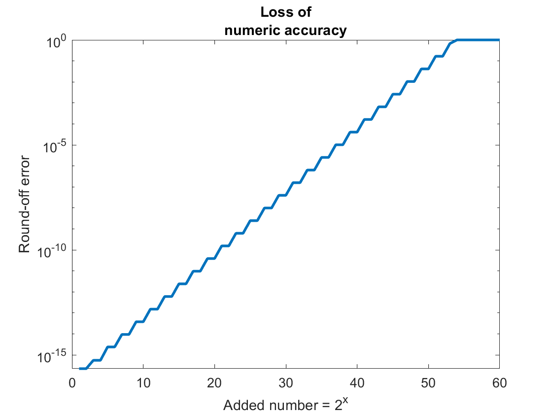
Fig. 2.21 The number a = 1.2 fills the full 52-bit significand allowed for double precision floating point numbers. As the number added to a gets larger, more of a is lost to round-off error.

2.9.2. Matrix Condition Number

Another problem besides round-off errors may degrade the accuracy of solutions to systems of equations. The symptom of the problem is an over-sensitivity to variations of the elements of \(\bm{b}\) when the system is nearly singular, which is also called poorly conditioned, or ill-conditioned. If the coefficients are taken from experiments, they likely contain a random component. We say there are perturbations to \(\bm{b}\). In many applications, \(\bf{A}\) is a fixed control matrix, so errors are more likely to be seen in \(\bm{b}\).

Errors in \(\bm{b}\), represented as \(\delta\bm{b}\), are conveyed to the solution \(\bm{x}\). The matrix equation \(\mathbf{A}\,\bm{x} = \bm{b}\) becomes \(\mathbf{A}\,\hat{\bm{x}} = \bm{b} + \delta\bm{b}\). Our estimate of the correct value of \(\bm{x}\) is \(\hat{\bm{x}} = \bm{x} + \bm{\delta x}\).

\[\begin{split}\begin{aligned} \mathbf{A}\,(\bm{x} + \bm{\delta x}) &= \bm{b} + \bm{\delta b} \\ \mathbf{A}\,\bm{x} + \mathbf{A}\,\bm{\delta x} &= \bm{b} + \bm{\delta b} \\ \mathbf{A}\,\bm{x} = \bm{b}, \quad &\text{and} \quad \mathbf{A}\,\bm{\delta x} = \bm{\delta b} \end{aligned}\end{split}\]

We care about the magnitudes of \(\bm{\delta x}\) and \(\bm{\delta b}\) relative to their true values. We want to find the length (norm) of each error vector relative to their unperturbed length, \(\norm{\bm{\delta x}} / \norm{\bm{x}}\) and \(\norm{\bm{\delta b}} / \norm{\bm{b}}\). We then have the following two inequalities because the norm of a product is less than or equal to the product of the norms of each variable.

(2.20)\[ \norm{\bm{\delta x}} \leq \norm{\mathbf{A}^{-1}}\, \norm{\bm{\delta b}} \qquad \frac{1}{\norm{\bm{x}}} \leq \norm{\mathbf{A}}\,\frac{1}{\norm{\bm{b}}}\]

Multiplying the two inequalities of equation (2.20) leads to equation (2.21).

(2.21)\[ \frac{\norm{\bm{\delta x}}}{\norm{\bm{x}}} \leq \norm{\mathbf{A}} \norm{\mathbf{A}^{-1}}\,\frac{\norm{\bm{\delta b}}}{\norm{\bm{b}}}\]

Equation (2.21) defines the condition number of \(\mathbf{A}\), which is a metric that relates the error in \(\bm{x}\) to the error in \(\bm{b}\). The condition number measures how well or poorly conditioned a matrix is. The condition of \(\bf{A}\) is denoted as \(\kappa({\mathbf{A}})\) [WATKINS10].

\[\frac{\norm{\bm{\delta x}}}{\norm{\bm{x}}} \leq \kappa(\mathbf{A})\, \frac{\norm{\bm{\delta b}}}{\norm{\bm{b}}}\]

(2.22)\[ \kappa(\mathbf{A}) = \text{cond}(\mathbf{A}) = \norm{\mathbf{A}}\norm{\mathbf{A}^{-1}}\]

Matrices that are close to singular have large condition numbers. If \(\kappa(\mathbf{A})\) is small, then small errors in \(\bm{b}\) results in only small errors in \(\bm{x}\). Whereas if \(\kappa(\mathbf{A})\) is large, then even small perturbations in \(\bm{b}\) can result in a large error in \(\bm{x}\). The condition number of the identity matrix and an orthogonal matrix is 1, but nearly singular matrices can have condition numbers of several thousand to even over a million.

The cond function in Python’s numpy.linalg module uses the \(\norm{\cdot}_2\) matrix norm by default, but may also compute the condition number using other matrix norms defined in Matrix Norms. MATLAB calculates the condition number using the singular values of the matrix as described in Condition Number. Using the singular values, there is a concern about division by zero, so MATLAB calculates the reciprocal, which it calls RCOND. Linear system solvers check the condition of a matrix before attempting to find a solution.

A handy rule of thumb for interpreting the condition number is if \(\kappa(\mathbf{A}) \approx 0.d \times 10^k\) then the solution \(\bm{x}\) can be expected to have \(k\) fewer digits of accuracy than the elements of \(\bf{A}\) [WILLIAMS14]. Thus, if \(\kappa(\mathbf{A}) = 10 = 0.1 \times 10^1\) and the elements of \(\bf{A}\) are given with six digits, then the solution in \(\bm{x}\) can be trusted to five digits of accuracy.

Here is an example to illustrate the problem. To be confident of the correct answer, we begin with a well-conditioned system.

(2.23)\[\begin{split}\left\{\begin{aligned} 17\,x_1 - 2\,x_2 &= -3 \\ -13\,x_1 + 29\,x_2 &= 29 \end{aligned}\right.\end{split}\]

It is easily confirmed with MATLAB that the solution is \(x_1 = -0.0621, x_2 = 0.9722\).

We assert that the system of equations in equation (2.23) is well-conditioned based on two pieces of information. First, the condition number of \(\bf{A}\) is a relatively small (2.3678). Secondly, minor changes to the equation have a minor impact on the solution. For example, if we add 1% of \(b_2\) to itself, we get a new solution of \(x_1 = -0.0609, x_2 = 0.9827\), which is a change of 2% to the solution \(x_1\) and 1.09% to \(x_2\).

Now, to illustrate a poorly conditioned system, we will alter the first equation of equation (2.23) to be the sum of the second equation and only \(1/100\) of itself.

(2.24)\[\begin{split}\left\{\begin{aligned} -12.83\,x_1 + 28.98\,x_2 &= 28.97 \\ -13\,x_1 + 29\,x_2 &= 29 \end{aligned}\right.\end{split}\]

Perhaps surprisingly, both LU decomposition and RREF can find the correct solution to equation (2.24). One can see that equation (2.24) is nearly singular because the two equations are close to parallel. The condition number is large (431). If we again add 1% of \(b_2\) to itself, we get a new solution of \(x_1 = -1.8617, x_2 = 0.1754\), which is a change to the \(x_1\) solution of 2,898%, and the \(x_2\) solution changed by 81.96%.

Another important result related to the condition number of matrices is that the condition number of the product of uncorrelated matrices is usually greater than the condition numbers of either of the individual matrices, and is sometimes equal to the product of the condition numbers of the individual matrices.

\[\kappa(\mathbf{A\,B}) = \norm{\mathbf{A\,B}}\,\norm{(\mathbf{A\,B})^{-1}} \leq \norm{\mathbf{A}}\, \norm{\mathbf{B}}\, \norm{\mathbf{B}^{-1}}\, \norm{\mathbf{A}^{-1}} = \kappa(\mathbf{A})\,\kappa(\mathbf{B})\]

In the next section (Orthogonal Matrix Decompositions), we multiply orthogonal matrices without increasing the condition number of the product because the condition number of an orthogonal matrix is 1.

2.9.3. The Case for Partial Pivoting

For numerical stability, very small numbers should not be used as pivot variables in the elimination procedure. Each time the pivot is advanced, the remaining rows are sorted to maximize the absolute value of the pivot variable. The new row order is documented with a permutation matrix to associate results with their unknown variable. Reordering rows, or row exchanges, is also called partial pivoting. Full pivoting is when columns are also reordered.

Here is an example showing why partial pivoting is needed for numerical stability. The example uses a \(2{\times}2\) matrix, where we could see some round-off error. The \(\epsilon\) value used in the example is taken to be a very small number. Remember that round-off errors will propagate and build when solving a larger system of equations. Without pivoting, we divide potentially large numbers by \(\epsilon\), producing even larger numbers. In algebra, we can avoid large numbers but get small numbers in different places. In either case, during the row operation phase of elimination, we add or subtract numbers of very different values, resulting in round-off errors. The accumulated round-off errors become especially problematic in the substitution phase, where the denominator of a division might be near zero.

\[\begin{split}\left\{\begin{aligned} \epsilon \,x_1 + 2\,x_2 &= 4 \\ 3\,x_1 - x_2 &= 7 \end{aligned}\right.\end{split}\]

\[\begin{split} \begin{bmatrix} \epsilon & 2 \\ 3 & -1 \end{bmatrix} \begin{bmatrix} x_1 \\ x_2 \end{bmatrix} = \begin{bmatrix} 4 \\ 7 \end{bmatrix}\end{split}\]

Regarding \(\epsilon\) as nearly zero relative to the other coefficients, we can use substitution to quickly see the approximate values of \(x_1\) and \(x_2\).

\[\begin{split}\begin{array}{rl} x_2 &\approx \frac{4}{2} = 2 \\ &\hfill\\ x_1 &\approx \frac{7 + 2}{3} = 3 \end{array}\end{split}\]

2.9.3.1. Elimination Without Partial Pivoting

If we don’t first exchange rows, we get the approximate value of \(x_2\) with some round-off error, but fail to find a correct value for \(x_1\).

\[\begin{split}\begin{bmatrix} \epsilon & 2 & 4 \\ 3 & -1 & 7 \end{bmatrix}\end{split}\]

Only one elimination step is needed.

\[\begin{split} \begin{bmatrix} \epsilon & 2 & 4 \\ 0 & {-(1 + \frac{6}{\epsilon})} & {(7 - \frac{12}{\epsilon})} \end{bmatrix}\end{split}\]

\[\left(1 + \frac{6}{\epsilon}\right) x_2 = \frac{12}{\epsilon} - 7\]

We could multiply both sides of the equation by \(\epsilon\) to simplify it, or calculate the fractions. In either case, the 1 and 7 terms will be largely lost to round-off error.

\[x_2 \approx \frac{12}{6} = 2\]

Our calculation of \(x_1\) is completely wrong. Getting the correct answer requires dividing two numbers that are close to zero.

\[\begin{split}\begin{array}{rl} &\epsilon x_1 + 2 x_2 = 4 \\ &\hfill\\ &\epsilon x_1 = 4 - 2 x_2 = 0 \\ &\hfill\\ &x_1 = \frac{4 - 2 x_2}{\epsilon} \approx \frac{0}{\epsilon} = 0 \end{array}\end{split}\]

2.9.3.2. Elimination With Partial Pivoting

Now we begin with the rows exchanged.

\[\begin{split}\begin{bmatrix} 3 & -1 & 7 \\ \epsilon & 2 & 4 \end{bmatrix}\end{split}\]

Again, only one elimination step is needed.

\[\begin{split} \begin{bmatrix} 3 & -1 & 7 \\ 0 & {(2 + \frac{\epsilon}{3})} & {(4 - \frac{7 \epsilon}{3})} \end{bmatrix}\end{split}\]

We will again lose some accuracy to round-off errors, but our small \(\epsilon\) values are paired with larger values by addition or subtraction and have minimal impact on the back substitution equations.

\[\begin{split}\begin{array}{rl} &x_2 \approx \frac{4}{2} = 2 \\ &\hfill \\ &3 x_1 - x_2 = 7 \\ &\hfill \\ &x_1 \approx \frac{7 + 2}{3} = 3 \end{array}\end{split}\]

Partial pivoting is used in both RREF and LU decomposition. It will use the small values in the calculation that we rounded to zero, so the results will be more accurate than our approximations.

In [5]: import numpy as np

In [6]: eps = 2.5e-16

In [7]: A = np.array([[3, -1], [eps, 2]])

In [8]: b = np.array([7, 4], dtype=float).T

In [9]: x = np.linalg.solve(A, b); x
Out[9]: array([3., 2.])

# not completely rounded
In [10]: np.all(x == np.array([3, 2]))
Out[10]: np.False_